The Third-to-Last Thing I’ll Ever Write About Expected Goals
Of all the positions I may or may not have about expected goals, the one that’s truly indefensible is to say there’s not much value in ExpG, then sit on the results as if it’s a set of nuclear launch codes.
So this is my model.
I should clarify that there isn’t one model per se1. Almost every time I build it, I’ll tweak the inputs. Usually that involves trying some different interactions. This time I added in a variable I had never used before. Woo hoo, free and fresh info! In the output below there is a variable for ‘interval’ that breaks the game down into 12 mostly equal time periods (one for every 7.5 minutes). So ‘interval1’ is from kickoff to 7 minutes 30 seconds; ‘interval2’ runs from 7:31 to 15:00. They aren’t precisely even because the last interval in each half (interval6, interval12) runs until the half- and full-time whistle (i.e. includes stoppage time). Moreover, I have left a few things out2 but for the most part this is roughly 85% (or more) of what I use every time I do an ExpG calculation. In fact most of the info in an ExpG calculation is in the shot location (there’s a visual of that here). If all you know is the distance to the goal from where the shot was taken, you can make a decent ExpG model.
Below is a list of the coefficients. Each of those numbers is a log odds-multiplier. So to turn that into something you can make sense of you have to do some math. Take one of the coefficient names. Let’s use ‘interval6’; that’s the last chunk of time up from 37:30 until the halftime whistle. Reading across, it has a coefficient of -1.375036e-02.
So you have to exponentiate that (and here ‘log’ is natural log). That means you take e to the -.01375036 power. Or: 2.7183 ^ -.01375036 (or 2.7183-.01375036).3 Oh, this last superscript isn’t re-raising to the power of 3, it’s for the footnote.
After exponentiating we get: .98634.
Then multiply the odds by that number. So, all things being equal, if we take a shot in the last 7.5 minutes of the first half, the odds the shot goes in decrease by about 1.37%. The size mightn’t be large, but the coefficient is significant (given our model selection criteria) and not completely surprising. You don’t want to concede right before half—well, you generally don’t want to concede ever. But teams are slightly more defensively minded so as not to give up a goal right before half and give up momentum and become dispirited or something. Maybe. It could be something completely different that we’re capturing. The math is only part of the equation, figuring out what the numbers actually mean is also pretty important (and sometimes the really hard thing to do).
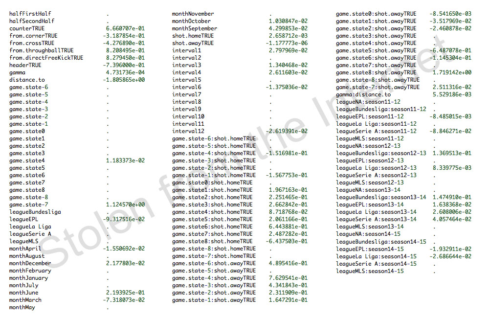
As an example of why I like interaction terms, I included season and league effects for all the leagues. So take “leagueBundesliga:season12-13” (which, if it’s not immediately obvious, is for the Bundesliga’s 2012-13 season). It has a coefficient of 1.369513e-01. Exponentiate and we get: 1.146772. That means the odds a shot taken in the Bundesliga in the 2012-13 season was scored as a goal increase 14.7%4. Why? I have no idea5. The following season was even more ‘lethal’. If you’ll notice there is also a variable that is just ‘Bundesliga’. It has no coefficient. However, if we take out the interaction between leagues and seasons and rebuild with just the leagues6, we get a ‘Bundesliga’ coefficient of 9.978884e-02.
So without season effects, we get an overall odds multiplier for Germany of about 1.105. But with season effects we can isolate that increase entirely to the 2012-13 and 2013-14 seasons (there are no coefficients for 2011-12 or 2014-15).
The coefficient names that probably aren’t self-evident are the ‘game.state’ variables. The game state is the score differential. It’s always the home team minus the visiting team. So if the home team is up 2-1 (or 3-2, etc.), the game state is 1. If the visiting team is leading 0-2 (or 1-3, etc.), the game state is -2. Shot.home and shot.away identify which team took the shot. So ‘game.state-2:shot.awayTRUE’ means the away team was up 2 goals and the away team took the shot (and the coefficient is curiously large; ~28% increase).
It’s easy to tell a plausible story about why this is happening. If you’re up 2 goals away, the home team is going to start pushing forward trying to score to get back in the game. That’s probably leaving them more exposed at the back. So there are more counter-attacking opportunities or just shots with fewer players in the box or whatever. Whether there is a way to exploit this without causing an increase in the corresponding ‘game.state-2:shot.homeTRUE’, that’s for a smarter person to figure out. Hopefully someone who manages a soccer team.
If you’re wondering how you turn this into an equation that lets you take a shot and assign a probability to it, you don’t. Not in any straightforward way. I am totally sympathetic if that annoys you. That’s where this came from in the first place. I was looking around online for something that would allow me to do an ExpG calculation but every model was either kept secret or was built in a way that I didn’t care for. I figured I could complain or just build my own. I chose the latter. Actually I probably did the former first, then realized it wasn’t as useful as doing the latter.
I spent a fair amount of time thinking about the best way to make the above results available. I could have posted an R file with step-by-step instructions on using it. But 1) that wouldn’t have given many people much insight to what was actually happening and 2) matching all the factor levels and getting input in the right format for the function to give you the proper output is a huge pain. It’s not conceptually difficult, but it’s super particular. I also thought about making an online tool that lets you put in the values and spits out a probability but that wouldn’t give you any idea what’s under the hood. Plus, navigating 20 different pulldowns and text input boxes to get back one number doesn’t seem like a great user experience (I might still do this with a model that uses just the shot location, but I also hate coding for the web).
So this seemed like the best approach to give some information that is robust and accessible. In other words, knowing that a given shot has, say, a .173 probability of being a goal isn’t nearly as interesting/useful as knowing that having an 0-2 lead on the road means the next shot has a much better chance (about 30%) of being a goal than if the same shot was taken at 0-07. The former might give me a better indication of what happened during a game than ‘shot was taken’, but the latter might give me some information I could use to help me win a game8.
1Moreover, when you run penalized regression this way, you are really creating a large set of candidate models, then doing model selection. Here I’m doing model selection using AICc. I could just as well use a different criterion and our coefficients would be slightly different. But once you have the dataset you can rejigger how you build the inputs and generate another set of candidate models in about 30 seconds (if you don’t screw something up, and I often do). Moreover, depending what went in on the front end, even using the same model-selection criteria we might get slightly different results. For example, if you do this using just Premier League data you actually get coefficients for the First Half and the Second Half (if I recall correctly it was a tiny increase in the first half (small increase in the odds a shot goes in) and about an equally large decrease in the second half (in total it was about a 3% difference)).
2 If you’re interested in the omissions. these are the things I have included in other models but don’t have here:
—Player category: I classified by position (forward, mid, defensive mid, defender). Strikers should be more lethal than defenders. This seems straightforward. Accurately classifying players was much messier than I anticipated.
—MLS: You’ll notice there are lines with ‘MLS’ in them, but there is no actual MLS data in the model. It was all pulled out. So why are those lines there? The original dataset was made with factor levels for multiple leagues, including MLS. So even when you don’t put any MLS data in, you still have to have factor levels for it or everything breaks. It’s not skewing results. There should be a period across from anything with “MLS” in it. Do not interpret that to mean that there is no positive/negative effect in MLS. Finishing in MLS is actually poor (at least mathematically). There is simply no MLS data here.
—Some interaction terms: I like interaction terms. Just for fun I sometimes run everything interacted with everything else. Most of the interactions have been edited out. Most but not all. There are season league and season interactions.
—Lots of really esoteric attempts at finding out what makes good teams good (see the final footnote for more on this). I tried all sorts of weird things here. For example I made time windows for all the different kickoff times. So you’re answering the question: “Does start time impact scoring?” (not really, save maybe in La Liga, but then all you are really doing is modeling the fact that Barcelona and Madrid have the most late kickoffs). Anyway, the vast majority of these were useless. A couple were interesting, but mostly still useless.
—Counter attacks: If you notice there is a variable for ‘counter’ in the model. So it is indeed in there. Just a note that I have a complicated set of conditionals for trying to determine this. I’m not sure how good it is, and it is almost certainly under-including things (so we’re missing some things that are probably counters; I took that tradeoff over including shots that didn’t happen against a totally exposed defense).
If that sounds like a non-trivial chunk of stuff, it’s really not. What’s here is most of what I use any time I rebuild.
3 If you’ve totally forgotten everything you ever learned in trigonometry and are still slightly confused about what to do, here is a screencast of me using a calculator to do the calculation.
4 If you’re wondering ‘relative to what?” I relevel all the factors so that none of them gets subsumed into the intercept. Basically, we’re saying relative to a league where there is no coefficient on its league-season.
5 I’d be interested to hear from someone who follows the Bundesliga to chime in with a theory here. But in general if you’re wondering what kind of things can make a difference, think about the change in the offside rule in the EPL this season. It’s likely that will lead to a more negative coefficient because a decent number of shots from really dangerous positions are going to be whistled back (or should be cough*Liverpool*cough).
6 I did this running a separate build—I simply removed the interaction term between league and season, leaving just the league—but the full list of coefficients isn’t posted here.
7 If all you want is to be able to look at a 0-2 loss and say that, by ExpG, a ‘score’ of 1.85 to .978 gives us a better understanding of what actually happened over 90 minutes in terms of quality of chances and that the home team was maybe ‘better’ and on most other days doesn’t lose by two goals, I have absolutely no problem with that. And my guess is when people set out to build an ExpG model that’s all they are intending to do.
8 So when I talk about doing prediction, this is more what I am referring to. Not predicting which players will regress to the mean (or describing what should have happened in the game), but being able to see what levers we can push to affect outcomes. Strictly speaking folks who called me out on Twitter for predicting a player would regress (that is quite literally a prediction) had a legit gripe given my lack of clarity about this. And maybe to head off any additional slings/arrows, again, one of my biggest problems with ExpG is that the biggest misses are with the best teams, so we’re failing to capture things that might help us figure out what leads to being better. Some of that could be a failure on my part. If I’m only modeling obvious inputs, then I’m limited by that. But, again, once I saw where I was missing most (the largest difference between actual and expected over full seasons) I tried all sorts or things to try to get even a tiny bit more signal on the Barcelonas of the world. I did not have much success.
Lastly, here are four seasons of player calculations for the EPL, La Liga, the Bundesliga and Serie A (there are only three seasons of Serie A). Circling back to the top, I’m not even sure which model this prediction set comes from. It predates the coefficients above, but it shouldn’t matter too much. Almost all of my models are currently residing somewhere around a Residual Deviance/Null Deviance of .80 to .82. It comes with no warrantees (I might have made a mistake aggregating). It’s only players with 20 shots or more in a season, so you can’t reconstruct entire team-seasons. If you find player duplicates, it’s most likely not a mistake but because either a player moved during the season, or there are two players that share a name. Lastly, it’s a csv (comma-seprated value file). You can open in in Excel, but Excel will almost certainly screw up some of the names and dates because Excel is pretty much the worst thing ever.